Lecture 2 - Andrej Karpathy's course
The source code is copied below (from a Marimo notebook) - in between the code blocks, I also added some notes which contain the extra information I parsed from multiple LLM reasoning efforts (NotebookLM + Gemini inside Colab)
{% include "../ai/lecture2.html" %}
import marimo as mo
import requests
import torch
import torch.nn.functional as F
import matplotlib.pyplot as plt # for making figures
We follow the lecture 2 of Andrej Karpathy's course and add some comments.
# Read dataset
url = 'https://raw.githubusercontent.com/karpathy/makemore/master/names.txt'
content_in_bytes = requests.get(url).content
words = content_in_bytes.decode('utf-8').split()
stoi (string-to-index) and itos (index-to-string) are simple mappings allowing for an easy conversion between integer and string representations. Note that the matrices (incl. embeddings) will always handle integers, not strings.
# Now we create index-mappings from chars to ints and back
chars = set()
for n in words:
    chars_from_name = [i for i in n]
    [chars.add(i) for i in chars_from_name]
chars = sorted(list(chars))
# char to index
stoi = {s:i+1 for i,s in enumerate(chars)}
stoi['.'] = 0
# {".": 0, "a": 1, etc}
# index to str
itos = {s:i for i,s in stoi.items()}
# {0: ".", 1: "a", etc}
Remember that we are trying to build a context (with length = 3) that will be used to predict a target character (Y). For example, for the word emma, we will have the following pairs X,y (note that we also use '.' as the special ending character) (note also that indices can be converted to the string representation via the itos mapping):
=> [0,0,0] -> [5] (i.e. ['.','.','.'] -> ['e'])
=> [0,0,5] -> [13] (i.e. ['.','.','e'] -> ['m'])
=> [0,5,13] -> [13] (i.e. ['.','e','m'] -> ['m'])
=> [5,13,13] -> [1] (i.e. ['e','m','m'] -> ['a'])
=> [13,13,1] -> [0] (i.e. ['m','m','a'] -> ['.'])
# ...
context_length = 3

def build_dataset(words: list[str], context_length: int = 3):

    X = []
    Y = []

    for w in words:
        context = [0]*context_length
        # we want context to grow with every char
        for char in w + '.':
            prev_chars = context
            target = char
            X.append(prev_chars)
            Y.append(stoi[target])
            idx_char = stoi[char]
            context = context[1:] + [idx_char]

    X = torch.tensor(X)
    Y = torch.tensor(Y)
    return X,Y
We do a trivial train-validation-test dataset split for later calculation of the loss and to determine whether we are overfitting the dataset.
# splitting train-test datasets -  we could have used sklearn
n1 = int(len(words)*0.8)
n2 = int(len(words)*0.9)
Xtr, Ytr = build_dataset(words[:n1])
Xdev, Ydev = build_dataset(words[n1:n2])
Xte, Yte = build_dataset(words[n2:])
 ](https://postimg.cc/21dJ1XsN)
Okay, let's break down this code snippet. This section represents the core training loop for a neural network model built using PyTorch.
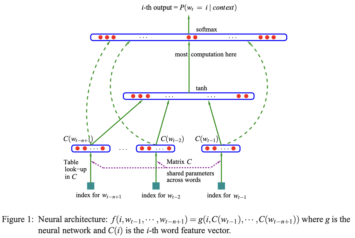
In essence, C acts as a table where you can "look up" the 10-dimensional feature vector (the embedding) associated with each of the 27 possible characters in your vocabulary. When an integer representing a character is fed into the model, this matrix is used to retrieve its corresponding 10-dimensional embedding vector, which then serves as input to the subsequent layers of the neural network.
Training Loop The code iterates 1000 times, performing the following steps in each iteration:
Minibatch Construction:
torch.randint: This function generates 32 random integers between 0 and the number of training examples (Xtr.shape[0]). These integers are stored in the ix variable.
ix: This variable acts as indices to select a random subset of the training data, forming a "minibatch" of size 32. Minibatches are used to make the training process more efficient.
Forward Pass:
emb = C[Xtr[ix]] # (32, 3, 2)
h = torch.tanh(emb.view(-1, 30) @ W1 + b1) # (32, 100)
logits = h @ W2 + b2 # (32, 27)
loss = F.cross_entropy(logits, Ytr[ix])
emb = C[Xtr[ix]]: This line retrieves the embeddings for the input data (Xtr) using the randomly selected indices (ix). Embeddings are numerical representations of the input data.
h = torch.tanh(emb.view(-1, 30) @ W1 + b1): This line performs a matrix multiplication between the reshaped embeddings and the weight matrix W1, adds a bias term b1, and then applies the hyperbolic tangent activation function (torch.tanh). This calculates the hidden state h of the neural network.
logits = h @ W2 + b2: This line performs another matrix multiplication between the hidden state h and the weight matrix W2, adds a bias term b2, resulting in the logits. Logits are the raw output of the neural network before applying any final activation function.
loss = F.cross_entropy(logits, Ytr[ix]): This line calculates the loss function, which measures the difference between the predicted output (logits) and the actual target values (Ytr[ix]). F.cross_entropy is a common loss function for classification tasks.
Backward Pass:
for p in parameters: p.grad = None: This loop resets the gradients of all model parameters (parameters) to zero. Gradients are used to update the parameters during training.
loss.backward(): This line performs backpropagation, calculating the gradients of the loss function with respect to all model parameters. This step is essential for optimizing the model's performance.
Update:
lr = 0.1 if i < 100000 else 0.01: This line sets the learning rate (lr). The learning rate controls the step size during parameter updates. In this case, a higher learning rate (0.1) is used initially, and then it is reduced to 0.01 after 100,000 iterations.
for p in parameters: p.data += -lr * p.grad: This loop updates the model parameters by subtracting the product of the learning rate and the gradient from the current parameter values. This process gradually adjusts the parameters to minimize the loss function.
Track Statistics:
stepi.append(i): This line records the current iteration number.
lossi.append(loss.log10().item()): This line records the logarithm (base 10) of the current loss value. Tracking these statistics allows monitoring the training progress and identifying potential issues.
g = torch.Generator().manual_seed(2147483647) # for reproducibility
C = torch.randn((27, 10), generator=g)
W1 = torch.randn((30, 200), generator=g)
b1 = torch.randn(200, generator=g)
W2 = torch.randn((200, 27), generator=g)
b2 = torch.randn(27, generator=g)
parameters = [C, W1, b1, W2, b2]
for param3 in parameters:
param3.requires_grad = True
print1 = False
stepi = []
lossi = []
for i in range(5000):
# mini batch
ix = torch.randint(0, Xtr.shape[0], (32,))
#ix = [i]
# forward pass
emb = C[Xtr[ix]]
mult = emb.view(-1,30) @ W1 + b1
h = torch.tanh(mult)
logits = h@W2 + b2
loss = F.cross_entropy(logits, Ytr[ix])
for param in parameters:
param.grad = None
loss.backward()
# update grads
lr = 0.1
for param2 in parameters:
param2.data += -lr * param2.grad
stepi.append(i)
lossi.append(loss.log10().item())
if print1 and i % 10:
print('Xtr', Xtr[ix])
print('emb', emb.shape)
print('mult', mult.shape)
print('h', h.shape)
print('logits', logits.shape)
print('Ytr', Ytr.shape)
print('loss', loss)
def calculate_loss(X, Y):
    emb1 = C[X]
    mult1 = emb1.view(-1,30) @ W1 + b1
    h1 = torch.tanh(mult1)
    logits1 = h1@W2 + b2
    loss1 = F.cross_entropy(logits1, Y)
    return loss1.item()
print('loss train', calculate_loss(Xtr, Ytr))
print('loss val', calculate_loss(Xdev, Ydev))
print('loss test', calculate_loss(Xte, Yte))
The embeddings are also plotted below (not displayed). Idea is that outliers (like "q" and ".") are distant from the cluster of the other letters, meaning that the network is able to learn that "q" has way fewer occurrances when analyzing names.